Learn Python From Zero For Absolute Beginner (1): Data cleaning

If you find yourself asking questions such as “What exactly does Python do?” or “How can I get started with Python”, then look no further than this handy guide. We understand that diving straight into code can feel intimidating, that’s why we focus on hands-on practice throughout this tutorial series, designed specifically for beginners.

No need to worry if you have never touched a single line of code before – we will take things slow at first and gradually build upon fundamental concepts. Let’s embark on this journey by starting with the first lesson below. Follow along with us!

In this article, you will learn how to perform the various data cleaning and manipulation tasks using Python.
Below are some of the examples:

While it is true that such tasks can be easily accomplished using Excel, this demonstration aims to familiarize you with the basics of Python in the context of a simple dataset.

By using Python, you can automate repetitive tasks, handle larger datasets more efficiently. This demo will introduce you to the fundamental concepts of data cleaning and manipulation in Python, empowering you to leverage its capabilities for more complex and specialized tasks beyond what can be achieved with Excel alone.

What you will learn in this article

• Basic concept of Python (e.g. data type, dataframe, etc.)
• Using Python to perform various data cleaning and manipulation
• Python Libraries “pandas”

Data source for this tutorial

In this tutorial, we will be using the “Year published” data in our “Chinese books before 1949 (Thread Bound)” collection. We hope that it could help you get to know a range of basic Python functions by playing around with this simple and straightforward data.

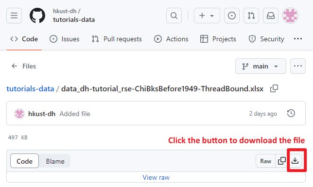
Let’s download the data here and get started with us now!

To ensure a seamless learning experience, we recommend you to create a new blank Jupyter Notebook and follow along with us step by step. While we have released a completed notebook on Google Colab, we encourage you to create a new notebook from scratch. If you are unsure how to create a new notebook on Google Colab, please refer to our previous article for detailed guidance.

While there are alternative tools like Anaconda or VS Code, we will be using Google Colab for demonstration. However, feel free to choose the environment that best suits your preferences and needs. The concepts and techniques we cover can be applied in any Python environment, and our goal is to facilitate your understanding of Python, regardless of the specific tools you use.

Let’s embark on this learning journey together and explore the power of Python!

Install Python Libraries

In this tutorial, we will focus on using a Python library called pandas (https://pandas.pydata.org/). It is one of the most popular and powerful libraries for data manipulation and analysis in Python, which provides a wide range of functions and methods to perform tasks such as data cleaning, filtering, aggregation, and more.

To use the functions and methods in pandas, we need to first install this library in our environment.
To do so, use the following syntax:

!pip install pandas

or you may need to use the following syntax instead in some environment:

import sys
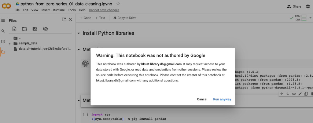
!{sys.executable} -m pip install pandas

PS: If you execute the code directly in the the Colab Notebook we provided, you will encounter the following warning message. No worries – simply click on “Run anyway” to proceed with running the cell.

Import Python Libraries

Then, import it by using the following line so that we can use the various functions and methods provided by the pandas library in the later part of our code.

import pandas as pd

Explanation
import pandas: import the pandas library
as pd: provide an alias or shorthand name for the imported library/module. In this case, we can simply type pd to call the pandas library’s functions later on instead of typing the full name pandas everytime.

Load data to Google Colab

If you are using tools like Anaconda or VS Code, you can skip this step of uploading the data file to Google Drive. Instead, save the data file you downloaded earlier on your computer. Ensure that the data file is saved in the same directory or folder as the notebook you created. By keeping them together, you will be able to easily access and load the data file within your Python code.

If you are using Google Colab like us, follow the steps below to upload the data file:

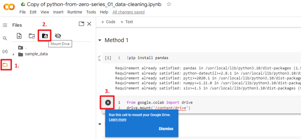
Method 1: Upload file to session storage

1. Click on the folder icon on the left-hand side of the Colab interface. This will open the file explorer panel.
2. Drag the data file to file explorer panel. This will upload the file to the Colab session storage.
3. You can then click the “Copy path” option to copy the file path and use it in the python code later.

Please note that the files you upload to Colab via this way will be stored in this temporary runtime. This runtime’s file will be deleted when this runtime is terminated – either by closing the browser tab or after a period of inactivity.

If you would like to have a more permanent location to retain the access to the data file beyond the current Colab session, please use Method 2 below.

Method 2: Use the file in your Google Drive

1. Click on the folder icon on the left-hand side of the Colab interface. This will open the file explorer panel.
2. Click the “Mount Drive” icon.
3. A cell that containing the drive.mount code will be appeared. Click the Run button to run the cell.

4. Choose an account to login and click “Connect to Google Drive” in order to allow Google Colab to access your Google Drive.

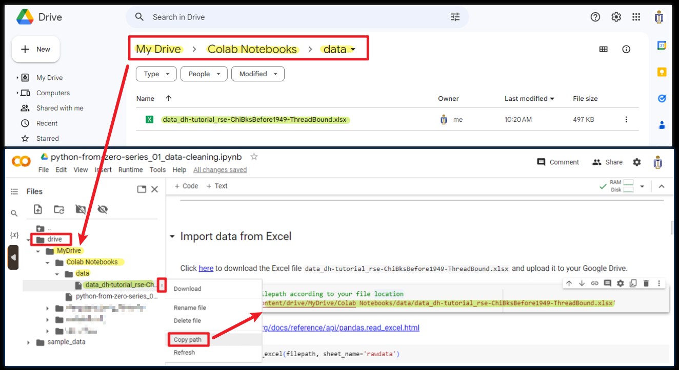
5. A “drive” folder will then be appeared in the file explorer panel. It will show all the files in your Google Drive.
6. Upload the data file to your Google Drive. You may upload it to anywhere you like in the Google Drive.
7. Expand the “drive” folder in the file explorer panel of Google Colab, find the file that you just uploaded. Click the dot icon on the right of the data file, and then click “Copy path” to copy the filepath of the file.
8. Paste the copied path to Colab notebook.

filepath = '/content/drive/MyDrive/Colab Notebooks/data/data_dh-tutorial_rse-ChiBksBefore1949-ThreadBound.xlsx'

In this example, we uploaded the file to the folder which named “data” inside the “Colab Notebooks” folder.
If you upload the file to the other location, for example, a folder called “testing_data” under “My Drive” directly, the copied path will then be /content/drive/MyDrive/testing_data/data_dh-tutorial_rse-ChiBksBefore1949-ThreadBound.xlsx

Import data from Excel / CSV

Use pandas.read_excel to read data from Excel file.
As we previously import the library using this line import pandas as pd, we can shortform pandas.read_excel to pd.read_excel .

filepath = '/content/drive/MyDrive/Colab Notebooks/data/data_dh-tutorial_rse-ChiBksBefore1949-ThreadBound.xlsx'
pd.read_excel(filepath, sheet_name='rawdata')

Tips: It is a good habit to check the documentation. At the beginning, you may feel overwhelmed because the documentation lists all methods related to a specific function. Just search the method you are using and read that part for a good starting point.

Documentation of pandas.read_excel :
https://pandas.pydata.org/docs/reference/api/pandas.read_excel.html

If your data file is in csv format, use pandas.read_csv :
https://pandas.pydata.org/pandas-docs/stable/reference/api/pandas.read_csv.html

In order to easily reuse the imported data, let’s add data = on the left-hand side of the code.
You can name it whatever you want. In this example, we named it as data.

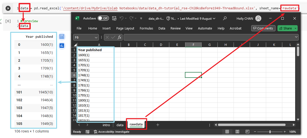
data = pd.read_excel(filepath, sheet_name='rawdata')

The result of the pd.read_excel is now assigned to the variable which named data. This means that the data from the Excel file is now stored in this variable.

Preview the data

In the previous step, we read the Excel file into a pandas DataFrame.

What is DataFrame?

DataFrame can be thought of as a table or spreadsheet-like data structure where data is organized into rows and columns.

We named this DataFrame as data. So, by typing data, we can preview its content.

data

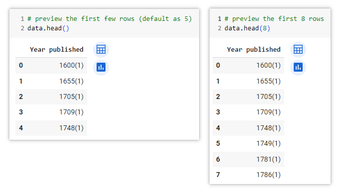
If a DataFrame has a large number of rows, using the .head() or .tail() method is a convenient way to view only the first or last few rows of the DataFrame. When you use them without specifying a number inside the parentheses, it defaults to displaying the first/last 5 rows of the dataset. You can input number inside the parentheses with any desired value to retrieve a different number of rows. For example .head(8) will display the first 8 rows.

This method is particularly useful when dealing with large datasets, as it allows you to get a quick glimpse of the data without displaying the entire DataFrame. It helps in quickly verifying the column names and identifying any potential issues or inconsistencies in the initial rows.

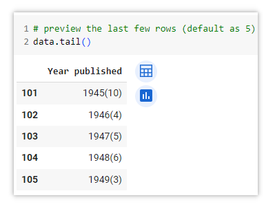
data.head()

data.tail()

Data cleaning

Now, let’s dive into using Python to perform some data cleaning and manipulation tasks.

Split one column to multiple columns according to special character

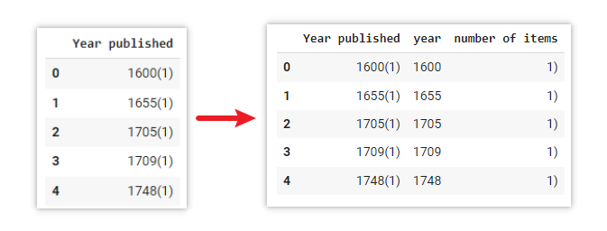
data[['year','number of items']] = data['Year published'].str.split('(',expand=True)

Explanation

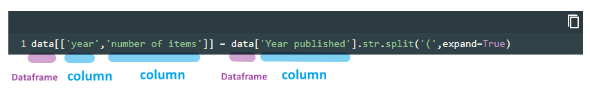
• data[[‘year’,’number of items’]]: Assign the result (right-hand side of the code) to new columns year and number of items in the data DataFrame

• data[‘Year published’]: Select the Year published column from the data DataFrame
• str: turns value in data[‘Year published’] into strings (i.e. text)
• split(‘(‘: Splits each value based on the left bracket symbol (
• expand=True: Expand the split strings into separate multiple columns

Documentation: https://pandas.pydata.org/docs/reference/api/pandas.Series.str.split.html

Remove columns

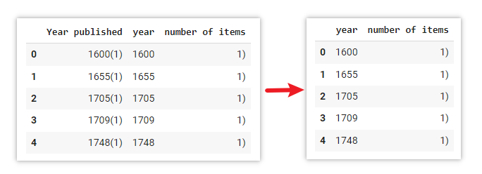
data = data.drop(columns=['Year published'])

Explanation
Use .drop() method to remove a specific column in the DataFrame.

Documentation: https://pandas.pydata.org/docs/reference/api/pandas.DataFrame.drop.html

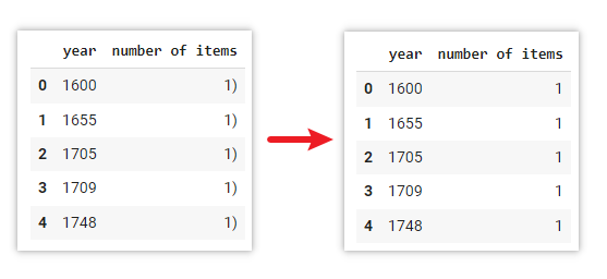
Replace specific character

data['number of items'] = data['number of items'].str.replace(')','')

Explanation
Use .replace() method to replace the right bracket symbol ) to empty character in the number of items column.

Documentation: https://pandas.pydata.org/docs/reference/api/pandas.DataFrame.replace.html

Check whether there is missing value

data.info()

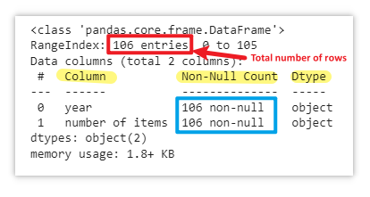
The .info() method provides a concise summary of the DataFrame, displaying information such as the column names, the count of non-null values for each column, and data type of each column.

By examining the output of the .info() method , you can quickly determine if there are missing values in your dataset. If a column has fewer non-null values compared to the total number of rows, it indicates the presence of missing or null values.

For example, if there are 106 entries (rows) in the dataset but only 105 non-null values, it means there is one missing value.

Documentation: https://pandas.pydata.org/docs/reference/api/pandas.DataFrame.info.html

Change data type of a column

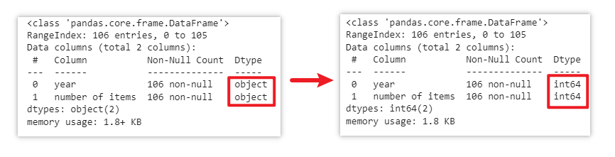
data['number of items'] = data['number of items'].astype('int')
data['year'] = data['year'].astype('int')
data.info()

Originally, the data type of the year and number of items columns is “object”. This means that the values in these columns are treated as strings or textual data, rather than numbers. In this case, we cannot use them to perform mathematical calculations. To ensure the data can be used for further analysis and computations, let’s convert it to int which means “integer” by using the .astype() method.

Documentation: https://pandas.pydata.org/docs/reference/api/pandas.DataFrame.astype.html

Commonly used Data Types

Descriptive statistics (get max and min values)

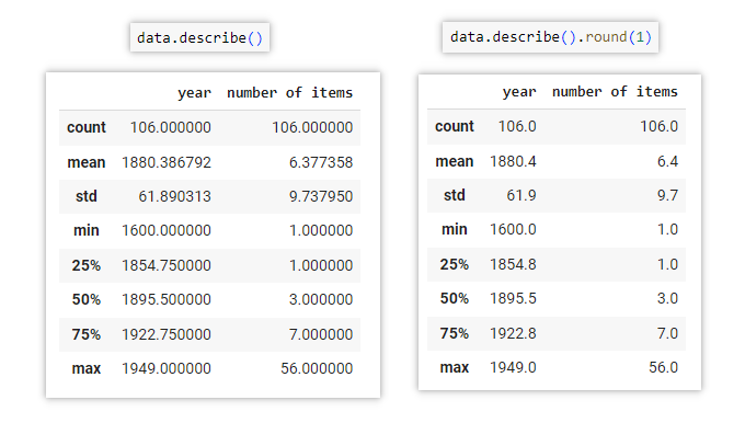
data.describe()

Documentation: https://pandas.pydata.org/docs/reference/api/pandas.DataFrame.describe.html

The .describe() method is used to generate descriptive statistics of a DataFrame. It provides summary statistics for each numerical column, such as count, mean, standard deviation, minimum, maximum, and quartiles.

For example, by referring to the min and max information generated via this method, we got to know that the earliest year and the latest year in this collection of data are in the range of 1600 to 1949.

data.describe().round(1)

We can also use .round() to round the values to a specified number of decimal places, improving the readability of the data, removing unnecessary decimals.

Documentation: https://pandas.pydata.org/docs/reference/api/pandas.DataFrame.round.html

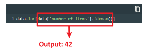
Get the row of maximum value (loc, idxmax)

data.loc[data['number of items'].idxmax()]

Output:
year 1884
number of items 56
Name: 42, dtype: int64

Let’s break down the code and understand its functionality:

.idxmax() returns the index label of the maximum value in the selected column. In other words, it finds the row where the number of items is the highest. In this case, row with index 42 has the highest number of items in this dataset.

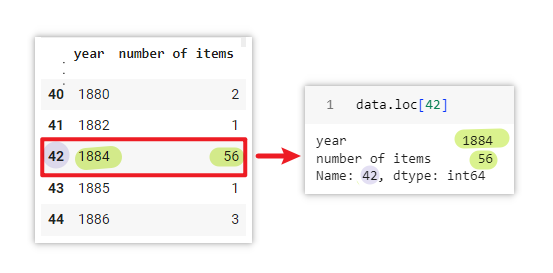
Let’s see what values are inside row index 42:

data.loc[42]

Output:
year 1884
number of items 56
Name: 42, dtype: int64

.loc[] is the indexing operator used to access rows and columns in a DataFrame. Here, it is used to access the row with the index label obtained from idxmax(). It retrieves the entire row based on the index label, including all the columns and their respective values. In this case, it selected row 42, which is the row where the number of items is the highest. For better understanding, the table below illustrates the returned output in row 42:

Retrieve element at index:

yearMaxItems = data.loc[data['number of items'].idxmax()]
print(yearMaxItems[0]) #Use print() to show the results in the output

Output: 1884

Explanation: This retrieves the element at index 0 in the yearMaxItems list. In Python, indexing starts from 0, so the first element in a list has an index of 0.

print(yearMaxItems[1])

Output: 56

Explanation: This retrieves the element at index 1 in the yearMaxItems list. Similarly, the second element in a list has an index of 1.

Documentation

• idxmax() : https://www.w3schools.com/python/pandas/ref_df_idxmax.asp
• loc[] : https://pandas.pydata.org/docs/reference/api/pandas.DataFrame.loc.html

Concatenation (combine string and variables)

Concatenation means merging/joining/combining multiple strings and variables together to create a single string.

In the example below, we try to combine the calculated sum value with some strings.

Let’s calculate the sum value first.
.sum() can be used to calculates the sum of the values.
Here, the sum of the number of items column in the data DataFrame is calculated.

sumvalue = data['number of items'].sum()
print(sumvalue)

Output: 676

Documentation: https://pandas.pydata.org/docs/reference/api/pandas.DataFrame.sum.html

Comma , , plus sign + and f string can be used to concatenate strings and variables together. They can achieve the same output result. See examples below.

print('There are a total of ', sumvalue, ' items in this collection.')

print('There are a total of ' + str(sumvalue) + ' items in this collection.')

print(f'There are a total of {sumvalue} items in this collection.')

Output: There are a total of 676 items in this collection.

print(f'Maximum: In this collection, there are {yearMaxItems[1]} items that were published in {yearMaxItems[0]}.')

Output: Maximum: In this collection, there are 56 items that were published in 1884.

Learn more here: https://pythonguides.com/concatenate-strings-in-python/

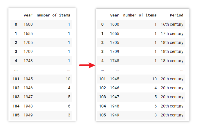
Assign labels to new column according to conditions (for loops, if…else)

From the output of .describe() earlier, we can observe that there are 106 unique years within the range of 1600 to 1949 in the data file. It contains a relatively large number of individual years within this time period.

To make it easier to interpret and understand the patterns, let’s group the years into broader time periods, such as “16th century”, “17th century”, “18th century”, etc.

Method 1

# create a function called "grouped_year"
def grouped_year(year):
  if 1501 <= year <= 1600:     # if the value of year is larger than or equal to 1501 AND smaller than or equal to 1600
    return "16th century"      # then, assign "16th century" to the "Period" column for this row
  elif 1601 <= year <= 1700:
    return "17th century"
  elif 1701 <= year <= 1800:
    return "18th century"
  elif 1801 <= year <= 1900:
    return "19th century"
  elif 1901 <= year <= 2000:
    return "20th century"
  else:
    return "Ungrouped"         # in case any values fall outside the above scope, show "Ungrouped" in the "Period" column for this row
# make a copy of the original dataframe "data", and named the copy as "data1"
data1 = data.copy()
# create a new column called "Period", and assign label to each row
data1["Period"] = data["year"].apply(lambda year: grouped_year(year))

Explanation
1. Create a function
A function called grouped_year is created. This function takes a year as input and assigns a category to it based on predefined ranges. For example, if the year falls between 1501 and 1600 (inclusive), it is considered part of the 16th century. Similarly, the function checks other ranges and assigns appropriate labels such as 17th century, 18th century, 19th century and 20th century. If a year doesn’t fall within any of these ranges, it is labeled as Ungrouped.

2. Make a copy of the DataFrame
To play safe, use .copy() to create a copy of a DataFrame. Then, the original DataFrame can remain unchanged. Any modifications made to the copied DataFrame do not impact the original data. This helps prevent unexpected and unintended changes to the original DataFrame.

3. Apply the function created in step 1 to the new column
data1["Period"]: A new column named Period is created in the copied DataFrame data1.
data["year"]: access the year column in the DataFrame data.
.apply(lambda year: grouped_year(year)): .apply() method is used to apply a function to each value in the year column of data. In this case, a lambda function is used to pass each individual year value to our previously created grouped_year() function.

Documentation:

• Functions (def): https://www.w3schools.com/python/python_functions.asp
• for loops: https://www.w3schools.com/python/python_for_loops.asp
• if…elif…else: https://www.w3schools.com/python/python_conditions.asp
• apply: https://pandas.pydata.org/docs/reference/api/pandas.DataFrame.apply.html
• lambda: https://www.w3schools.com/python/python_lambda.asp

Method 2

You may also use the following 1 line of code to achieve the same output result:

# make a copy of the original dataframe "data", and named the copy as "data2"
data2 = data.copy()
# create a new column called "Period", and assign label to each row
data2['Period'] = ['16th century' if 1501 <= year <= 1600 else '17th century' if 1601 <= year <= 1700 else '18th century' if 1701 <= year <= 1800 else '19th century' if 1801 <= year <= 1900 else '20th century' if 1901 <= year <= 2000 else "Ungrouped" for year in data['year']]

Explanation
Same as Method 1, this line of code iterates over each value in the year column of the DataFrame data.
For each year value, the code checks a series of conditions using if…else statements.
The resulting values are collected in a list, which is then assigned to the Period column of data2.

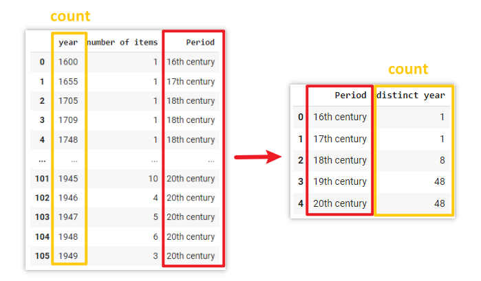
Group data (similar to pivot table in Excel)

# make a copy of the dataframe "data2", and named the copy as "data_r1"
data_r1 = data2.copy()

# find the number of distinct year in each period
data_r1 = data_r1.groupby('Period')['year'].count().reset_index()

# rename the column "year" to "distinct year"
data_r1.rename(columns={'year':'distinct year'}, inplace=True)

Explanation
The .groupby() method in Python is similar to the pivot table function in Excel which allows you to group and aggregate data based on specific columns.
In this example, it groups the data based on the unique values in the Period column, and counts the number of occurrences of the the values in the year column within each group.

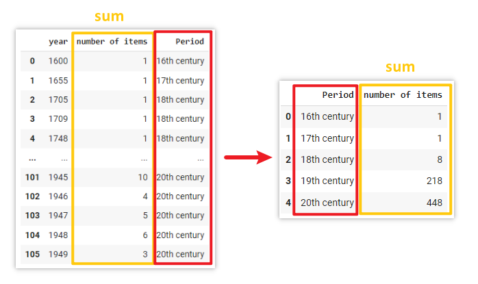
# make a copy of the dataframe "data2", and named the copy as "data_r2"
data_r2 = data2.copy()

# find the sum of number of items in each period
data_r2 = data_r2.groupby('Period')['number of items'].sum().reset_index()

Explanation
In this example, it groups the data based on the unique values in the Period column, and calculates the sum of the values in the number of items column for each group.

Documentation: https://pandas.pydata.org/docs/reference/api/pandas.DataFrame.groupby.html

Merge two tables/dataframes

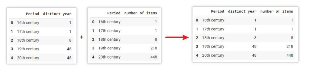
# Merge two DataFrame based on a particular column
data_r_merge = pd.merge(data_r1, data_r2, on='Period')

Explanation
The .merge() function in pandas can combine multiple dataframes together.
In this example, DataFrame data_r1 and data_r2 are combined into one DataFrame data_r_merge based on the Period column. The merge operation will match rows from both DataFrames that have the same values in the Period column.

There are more ways to merge, join, concatenate and compare between multiple DataFrames. Read the documentation to learn more: https://pandas.pydata.org/docs/user_guide/merging.html

Conclusion

As we reach the end of this article, we hope that it has provided you with a basic understanding of fundamental Python functions by working with the examples presented here. We encourage you to embark on your own exploration of Python’s possibilities and discover how it can be applied in various scenarios. Keep exploring the vast possibilities that Python could offer!

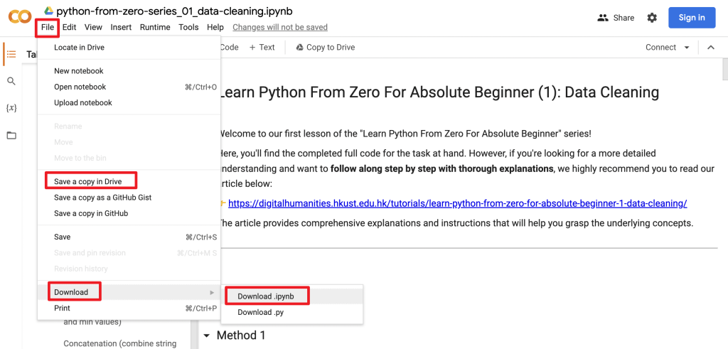
You may download or save a copy of our completed notebook on Google Colab. It consolidated all the code mentioned throughout this article.

Next article – Data Visualization

Moving forward, we invite you to join us in our next article, where we will embark on the journey into the realm of data visualization. Together, we will explore the powerful capabilities of Python for creating interactive charts and graphs. These visualizations will enable you to gain deeper insights into your data. Stay tuned for our upcoming article!

– By Holly Chan, Library

August 24, 2023

You may also be interested in…

Learn Python From Zero For Absolute Beginner (2): Data visualization

Read More

Learn Python From Zero For Absolute Beginner (3): Create Website

Read More

Turn your Jupyter Notebook into interactive Presentation Slides using Anaconda

Read More